Batch machine learning pipeline¶

OUTLINE:¶

• dataset preprocessing
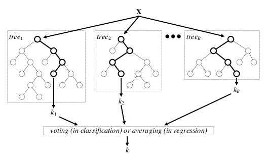
• classification pipeline - Random Forest
• results improvement
• feautre engineering
  dataset : TEP

Random Forest¶

[1] Verikas, Antanas, et al. "Electromyographic patterns during golf swing: Activation sequence profiling and prediction of shot effectiveness." Sensors 16.4 (2016): 592.

libraries¶

In [1]:

from sklearn.metrics import classification_report
from sklearn.metrics import confusion_matrix
from sklearn.model_selection import train_test_split
from skfeature.function.similarity_based import lap_score
from sklearn.preprocessing import StandardScaler, MinMaxScaler, RobustScaler
from sklearn.model_selection import cross_val_score
from sklearn.model_selection import GridSearchCV
from sklearn.ensemble import RandomForestClassifier
from sklearn.impute import SimpleImputer

#import xgboost

from imblearn.under_sampling import RandomUnderSampler
from imblearn.over_sampling import RandomOverSampler
from imblearn.pipeline import Pipeline

import glob
import pandas as pd
import numpy as np
from random import randrange

import seaborn as sns
import matplotlib.pyplot as plt
from mpl_toolkits.axes_grid1 import make_axes_locatable

import warnings
warnings.filterwarnings('ignore')
%matplotlib inline

from sklearn.metrics import classification_report from sklearn.metrics import confusion_matrix from sklearn.model_selection import train_test_split from skfeature.function.similarity_based import lap_score from sklearn.preprocessing import StandardScaler, MinMaxScaler, RobustScaler from sklearn.model_selection import cross_val_score from sklearn.model_selection import GridSearchCV from sklearn.ensemble import RandomForestClassifier from sklearn.impute import SimpleImputer #import xgboost from imblearn.under_sampling import RandomUnderSampler from imblearn.over_sampling import RandomOverSampler from imblearn.pipeline import Pipeline import glob import pandas as pd import numpy as np from random import randrange import seaborn as sns import matplotlib.pyplot as plt from mpl_toolkits.axes_grid1 import make_axes_locatable import warnings warnings.filterwarnings('ignore') %matplotlib inline

Create a Workshop TEP dataset wih imbalanced classes for batch learning¶

In [66]:

# drop_indices = []
# for fault in dataset['fault_id'].unique():
#     min_index = dataset[dataset['fault_id']==fault].index.min()
#     max_index = dataset[dataset['fault_id']==fault].index.max()
#     a = randrange(min_index, max_index)
#     b = randrange(min_index, max_index)
#     if a<b:
#         to_drop = np.arange(a,b)
#     else:
#         to_drop = np.arange(b,a)
#     drop_indices.extend(to_drop)

# drop_indices = [] # for fault in dataset['fault_id'].unique(): # min_index = dataset[dataset['fault_id']==fault].index.min() # max_index = dataset[dataset['fault_id']==fault].index.max() # a = randrange(min_index, max_index) # b = randrange(min_index, max_index) # if a

In [68]:

# dataset = pd.read_csv('dataset.csv', index_col=False)
# dataset.drop(drop_indices).to_csv('workshop_dataset.csv', index=False)
# dataset.iloc[drop_indices].to_csv('workshop_dataset_stream_testing.csv', index=False)

# dataset = pd.read_csv('dataset.csv', index_col=False) # dataset.drop(drop_indices).to_csv('workshop_dataset.csv', index=False) # dataset.iloc[drop_indices].to_csv('workshop_dataset_stream_testing.csv', index=False)

1. Preprocessing¶

In [2]:

dataset = pd.read_csv('workshop_dataset.csv',index_col=False)
col_names = dataset.columns.tolist()

dataset = pd.read_csv('workshop_dataset.csv',index_col=False) col_names = dataset.columns.tolist()

In [3]:

fig, ax = plt.subplots(8,7, figsize=(18, 18))
[fig.delaxes(ax[7,i]) for i in [3,4,5,6]]
ax = np.delete(ax.flatten(), [52,53,54,55])
dataset.boxplot(ax=ax, by='fault_id', rot=90, showfliers=False)
[ax.set_xlabel('') for ax in ax.flatten()[:-7]]
[ax.set_xticklabels([]) for ax in ax.flatten()[:-7]]
fig.subplots_adjust(hspace = 0.3, wspace=0.3)
fig.suptitle("TEP dataset feature boxplots, subplot=feature per fault_id", size=30, y=0.95);

fig, ax = plt.subplots(8,7, figsize=(18, 18)) [fig.delaxes(ax[7,i]) for i in [3,4,5,6]] ax = np.delete(ax.flatten(), [52,53,54,55]) dataset.boxplot(ax=ax, by='fault_id', rot=90, showfliers=False) [ax.set_xlabel('') for ax in ax.flatten()[:-7]] [ax.set_xticklabels([]) for ax in ax.flatten()[:-7]] fig.subplots_adjust(hspace = 0.3, wspace=0.3) fig.suptitle("TEP dataset feature boxplots, subplot=feature per fault_id", size=30, y=0.95);

In [4]:

fig, ax = plt.subplots(1, 1, figsize=(18, 3), facecolor='w', edgecolor='k')
fig.suptitle('Sample count per fault_id', size=20, y=1.12)
sns.countplot(ax = ax, x='fault_id', data=dataset,color='navy');

fig, ax = plt.subplots(1, 1, figsize=(18, 3), facecolor='w', edgecolor='k') fig.suptitle('Sample count per fault_id', size=20, y=1.12) sns.countplot(ax = ax, x='fault_id', data=dataset,color='navy');

1.2. Class imbalance impact¶

In [5]:

# define undersample strategy
# https://imbalanced-learn.readthedocs.io/en/stable/generated/imblearn.under_sampling.RandomUnderSampler.html
# 'not minority' = resample all classes to the size of minority class
undersample = RandomUnderSampler(sampling_strategy='not minority')
oversample = RandomOverSampler(sampling_strategy='not majority')

dataset_under_values, labels_under = undersample.fit_resample(dataset.drop(columns=['fault_id']), dataset['fault_id'])
dataset_under = pd.DataFrame(np.concatenate([dataset_under_values, labels_under.reshape(-1,1)], axis=1), columns = col_names)
dataset_under['type'] = 'under'
dataset_over_values, labels_over = oversample.fit_resample(dataset.drop(columns=['fault_id']), dataset['fault_id'])
dataset_over = pd.DataFrame(np.concatenate([dataset_over_values, labels_over.reshape(-1,1)], axis=1), columns = col_names)
dataset_over['type'] = 'over'

dataset['type'] = 'original'

# define undersample strategy # https://imbalanced-learn.readthedocs.io/en/stable/generated/imblearn.under_sampling.RandomUnderSampler.html # 'not minority' = resample all classes to the size of minority class undersample = RandomUnderSampler(sampling_strategy='not minority') oversample = RandomOverSampler(sampling_strategy='not majority') dataset_under_values, labels_under = undersample.fit_resample(dataset.drop(columns=['fault_id']), dataset['fault_id']) dataset_under = pd.DataFrame(np.concatenate([dataset_under_values, labels_under.reshape(-1,1)], axis=1), columns = col_names) dataset_under['type'] = 'under' dataset_over_values, labels_over = oversample.fit_resample(dataset.drop(columns=['fault_id']), dataset['fault_id']) dataset_over = pd.DataFrame(np.concatenate([dataset_over_values, labels_over.reshape(-1,1)], axis=1), columns = col_names) dataset_over['type'] = 'over' dataset['type'] = 'original'

In [6]:

fig, ax = plt.subplots(1, 1, figsize=(18, 3), facecolor='w', edgecolor='k')
fig.suptitle('Sample count per fault_id', size=20, y=1.12)
sns.countplot(ax = ax, x='fault_id', data=pd.concat([dataset, dataset_under, dataset_over], ignore_index=True), hue='type');

fig, ax = plt.subplots(1, 1, figsize=(18, 3), facecolor='w', edgecolor='k') fig.suptitle('Sample count per fault_id', size=20, y=1.12) sns.countplot(ax = ax, x='fault_id', data=pd.concat([dataset, dataset_under, dataset_over], ignore_index=True), hue='type');

In [7]:

def scale_dataset(dataset):
    scaler = StandardScaler()
    scaler.fit(dataset.drop(columns=['fault_id', 'type']))
    dataset_scaled = pd.DataFrame(scaler.transform(dataset.drop(columns=['fault_id', 'type'])),columns=col_names[:-1])
    dataset_scaled['fault_id'] = dataset['fault_id'].copy()
    return dataset_scaled

def scale_dataset(dataset): scaler = StandardScaler() scaler.fit(dataset.drop(columns=['fault_id', 'type'])) dataset_scaled = pd.DataFrame(scaler.transform(dataset.drop(columns=['fault_id', 'type'])),columns=col_names[:-1]) dataset_scaled['fault_id'] = dataset['fault_id'].copy() return dataset_scaled

In [8]:

feature = 'xmeas_3'
ds = dataset.copy()

fig, ax = plt.subplots(1,2, figsize=(18, 3))
ds[[feature, 'fault_id']].boxplot(ax=ax[0], rot=90, by='fault_id', showfliers=False)
scale_dataset(ds)[[feature, 'fault_id']].boxplot(ax=ax[1], rot=90, by='fault_id', showfliers=False)
fig.suptitle("TEP dataset feature scaling boxplots", size=20, y=1.1);

feature = 'xmeas_3' ds = dataset.copy() fig, ax = plt.subplots(1,2, figsize=(18, 3)) ds[[feature, 'fault_id']].boxplot(ax=ax[0], rot=90, by='fault_id', showfliers=False) scale_dataset(ds)[[feature, 'fault_id']].boxplot(ax=ax[1], rot=90, by='fault_id', showfliers=False) fig.suptitle("TEP dataset feature scaling boxplots", size=20, y=1.1);

2. Classification pipeline¶

2.1. Pipeline¶

In [9]:

pipe = Pipeline([('balancer',RandomOverSampler()), 
                 ('scaler', StandardScaler()), 
                 ('classifier', RandomForestClassifier())])
#('imputer', SimpleImputer(missing_values=np.nan, strategy='mean'))

pipe = Pipeline([('balancer',RandomOverSampler()), ('scaler', StandardScaler()), ('classifier', RandomForestClassifier())]) #('imputer', SimpleImputer(missing_values=np.nan, strategy='mean'))

2.2. Results¶

In [10]:

X = dataset.dropna().drop(columns=['fault_id','type'])
Y = dataset.dropna()['fault_id']
scores = cross_val_score(pipe, X, Y, cv=10)
print('10-Cross-Validation scores :\n' + str(scores))

X_train, X_test, Y_train, Y_test = train_test_split(X, Y, test_size=0.1)
pipe.fit(X_train, Y_train)
feature_importances = pipe.named_steps['classifier'].feature_importances_
print('Classification report :\n' + str(classification_report(Y_test, pipe.predict(X_test))))

X = dataset.dropna().drop(columns=['fault_id','type']) Y = dataset.dropna()['fault_id'] scores = cross_val_score(pipe, X, Y, cv=10) print('10-Cross-Validation scores :\n' + str(scores)) X_train, X_test, Y_train, Y_test = train_test_split(X, Y, test_size=0.1) pipe.fit(X_train, Y_train) feature_importances = pipe.named_steps['classifier'].feature_importances_ print('Classification report :\n' + str(classification_report(Y_test, pipe.predict(X_test))))

10-Cross-Validation scores :
[0.59202756 0.70246305 0.68506654 0.52       0.31472332 0.64950495
 0.67178218 0.65923725 0.68037661 0.70223325]
Classification report :
              precision    recall  f1-score   support

           0       0.50      0.29      0.36         7
           1       0.94      0.88      0.91       130
           2       0.93      0.87      0.90       134
           3       0.43      0.66      0.52       113
           4       0.90      0.89      0.89       149
           5       0.63      0.73      0.68       105
           6       0.95      0.92      0.93       144
           7       1.00      1.00      1.00        74
           8       0.91      0.92      0.92       147
           9       0.56      0.60      0.58        93
          10       0.75      0.80      0.77       128
          11       0.86      0.68      0.76        28
          12       0.97      0.95      0.96        96
          13       1.00      0.99      0.99        97
          14       0.93      0.83      0.88       115
          15       0.54      0.45      0.49        91
          16       0.89      0.80      0.84        49
          17       0.90      0.93      0.91        68
          18       1.00      0.80      0.89        10
          19       0.83      0.77      0.80        62
          20       0.91      0.74      0.82       121
          21       0.97      0.98      0.98        63

    accuracy                           0.82      2024
   macro avg       0.83      0.79      0.81      2024
weighted avg       0.84      0.82      0.83      2024

3. Improving results¶

3.1. Results Analysis¶

In [11]:

ds = scale_dataset(dataset)
fault_id = 1

fig, ax = plt.subplots(1,1, figsize=(18, 3))
ds[ds['fault_id']==fault_id].drop(columns=['fault_id']).boxplot(ax=ax, rot=90, showfliers=False)
fig.suptitle('Features values for fault_id : ' + str(fault_id), size=10);

ds = scale_dataset(dataset) fault_id = 1 fig, ax = plt.subplots(1,1, figsize=(18, 3)) ds[ds['fault_id']==fault_id].drop(columns=['fault_id']).boxplot(ax=ax, rot=90, showfliers=False) fig.suptitle('Features values for fault_id : ' + str(fault_id), size=10);

3.2. Parameter calibration¶

In [ ]:

# "classifier__" string same as in pipeline
param_grid = [{'classifier__n_estimators': [100, 200, 500],
               'classifier__max_features': ['auto', 'log2'],
               'classifier__max_depth' : [5,10,50,100,None],
               'classifier__criterion' :['gini', 'entropy']}]

RF_clf_gs = GridSearchCV(pipe, param_grid=param_grid, scoring='f1_weighted',n_jobs=4, cv=10)
RF_clf_gs.fit(dataset.drop(columns=['fault_id','type']), dataset['fault_id'])
means = RF_clf_gs.cv_results_['mean_test_score']
stds = RF_clf_gs.cv_results_['std_test_score']
print('RF 10CV f1 score mean with 95% confidence interval : ')
for mean, std, params in zip(means, stds, RF_clf_gs.cv_results_['params']):
    print("%0.3f (+/-%0.03f) for %r" % (mean, std * 2, params))

# "classifier__" string same as in pipeline param_grid = [{'classifier__n_estimators': [100, 200, 500], 'classifier__max_features': ['auto', 'log2'], 'classifier__max_depth' : [5,10,50,100,None], 'classifier__criterion' :['gini', 'entropy']}] RF_clf_gs = GridSearchCV(pipe, param_grid=param_grid, scoring='f1_weighted',n_jobs=4, cv=10) RF_clf_gs.fit(dataset.drop(columns=['fault_id','type']), dataset['fault_id']) means = RF_clf_gs.cv_results_['mean_test_score'] stds = RF_clf_gs.cv_results_['std_test_score'] print('RF 10CV f1 score mean with 95% confidence interval : ') for mean, std, params in zip(means, stds, RF_clf_gs.cv_results_['params']): print("%0.3f (+/-%0.03f) for %r" % (mean, std * 2, params))

3.3. Feature Engineering¶

3.3.1. Feature Selection¶

3.3.1.1. Feature importance (RandomForest, XGBoost)¶

In [79]:

feature_names = [col_names[i] for i in np.argsort(feature_importances)]

fig, ax = plt.subplots(1, 1, figsize=(16, 5))
fig.suptitle('Sorted features by their importance in Random Forest classifier', size=20)
ax.bar(np.arange(len(feature_importances)), np.sort(feature_importances)[::-1])
ax.tick_params(labelsize=10)
ax.set_xlim([-0.5, len(feature_importances)-0.5])
ax.set_xticks(np.arange(len(feature_importances)))
ax.set_xticklabels(feature_names[::-1], rotation=90);

feature_names = [col_names[i] for i in np.argsort(feature_importances)] fig, ax = plt.subplots(1, 1, figsize=(16, 5)) fig.suptitle('Sorted features by their importance in Random Forest classifier', size=20) ax.bar(np.arange(len(feature_importances)), np.sort(feature_importances)[::-1]) ax.tick_params(labelsize=10) ax.set_xlim([-0.5, len(feature_importances)-0.5]) ax.set_xticks(np.arange(len(feature_importances))) ax.set_xticklabels(feature_names[::-1], rotation=90);

3.3.1.2. Feature correlation¶

In [80]:

def corr_heatmap(dataset, title):
    fig, ax = plt.subplots(1, 1, figsize=(10, 10))
    fig.suptitle(title, size=20);
    heatmap = ax.matshow(dataset, cmap=plt.cm.seismic)
    ax.set_xticks(range(dataset.shape[1]))
    ax.set_xticklabels(dataset.columns.values, fontsize=10, rotation=90)
    ax.set_yticks(range(dataset.shape[0]))
    ax.set_yticklabels(dataset.index.values, fontsize=10)

    ax.set_xticks(np.arange(-.5, dataset.shape[1]-1, 1), minor=True);
    ax.set_yticks(np.arange(-.5, dataset.shape[0]-1, 1), minor=True);
    ax.grid(which='minor', color='w', linestyle='-', linewidth=2.)

    # create an axes on the right side of ax. The width of cax will be 5%
    # of ax and the padding between cax and ax will be fixed at 0.05 inch.
    divider = make_axes_locatable(ax)
    cax = divider.append_axes("right", size="2%", pad=0.1)

    cb = fig.colorbar(heatmap, cax=cax)
    cb.ax.tick_params(labelsize=12)
    
# do not correlate fault_ids and type :)
ds = dataset.copy()
dataset_corr = ds.drop(columns=['fault_id', 'type']).corr()
corr_heatmap(dataset_corr, 'Correlation matrix');

def corr_heatmap(dataset, title): fig, ax = plt.subplots(1, 1, figsize=(10, 10)) fig.suptitle(title, size=20); heatmap = ax.matshow(dataset, cmap=plt.cm.seismic) ax.set_xticks(range(dataset.shape[1])) ax.set_xticklabels(dataset.columns.values, fontsize=10, rotation=90) ax.set_yticks(range(dataset.shape[0])) ax.set_yticklabels(dataset.index.values, fontsize=10) ax.set_xticks(np.arange(-.5, dataset.shape[1]-1, 1), minor=True); ax.set_yticks(np.arange(-.5, dataset.shape[0]-1, 1), minor=True); ax.grid(which='minor', color='w', linestyle='-', linewidth=2.) # create an axes on the right side of ax. The width of cax will be 5% # of ax and the padding between cax and ax will be fixed at 0.05 inch. divider = make_axes_locatable(ax) cax = divider.append_axes("right", size="2%", pad=0.1) cb = fig.colorbar(heatmap, cax=cax) cb.ax.tick_params(labelsize=12) # do not correlate fault_ids and type :) ds = dataset.copy() dataset_corr = ds.drop(columns=['fault_id', 'type']).corr() corr_heatmap(dataset_corr, 'Correlation matrix');

3.3.1.3. Feature correlation - Improved¶

In [81]:

ds = dataset.copy()
dataset_corr = ds.drop(columns=['fault_id', 'type']).corr()
correlation_threshold = 0.8

upper = dataset_corr.where(np.triu(np.ones(dataset_corr.shape), k = 1).astype(np.bool))
# Select the features with correlations above the threshold
# absolute value - positive/negative correlation
to_drop = [column for column in upper.columns if any(upper[column].abs() > correlation_threshold)]

# Dataframe to hold correlated pairs
dataset_collinear = pd.DataFrame(columns = ['drop_feature', 'corr_feature', 'corr_value'])

# Iterate through the "columns to drop" to record pairs of correlated features
for column in to_drop:

    # Find the correlated features
    corr_features = list(upper.index[upper[column].abs() > correlation_threshold])

    # Find the correlated values
    corr_values = list(upper[column][upper[column].abs() > correlation_threshold])
    drop_features = [column for _ in range(len(corr_features))]    

    # Record the information (need a temp df for now)
    temp_df = pd.DataFrame.from_dict({'drop_feature': drop_features,
                                     'corr_feature': corr_features,
                                     'corr_value': corr_values})
    dataset_collinear = dataset_collinear.append(temp_df, ignore_index = True)
    
dataset_corr_filtered = dataset_corr.loc[list(set(dataset_collinear['corr_feature'])), list(set(dataset_collinear['drop_feature']))]

corr_heatmap(dataset_corr_filtered, 'Correlation matrix above threshold = ' + str(correlation_threshold));

ds = dataset.copy() dataset_corr = ds.drop(columns=['fault_id', 'type']).corr() correlation_threshold = 0.8 upper = dataset_corr.where(np.triu(np.ones(dataset_corr.shape), k = 1).astype(np.bool)) # Select the features with correlations above the threshold # absolute value - positive/negative correlation to_drop = [column for column in upper.columns if any(upper[column].abs() > correlation_threshold)] # Dataframe to hold correlated pairs dataset_collinear = pd.DataFrame(columns = ['drop_feature', 'corr_feature', 'corr_value']) # Iterate through the "columns to drop" to record pairs of correlated features for column in to_drop: # Find the correlated features corr_features = list(upper.index[upper[column].abs() > correlation_threshold]) # Find the correlated values corr_values = list(upper[column][upper[column].abs() > correlation_threshold]) drop_features = [column for _ in range(len(corr_features))] # Record the information (need a temp df for now) temp_df = pd.DataFrame.from_dict({'drop_feature': drop_features, 'corr_feature': corr_features, 'corr_value': corr_values}) dataset_collinear = dataset_collinear.append(temp_df, ignore_index = True) dataset_corr_filtered = dataset_corr.loc[list(set(dataset_collinear['corr_feature'])), list(set(dataset_collinear['drop_feature']))] corr_heatmap(dataset_corr_filtered, 'Correlation matrix above threshold = ' + str(correlation_threshold));

3.3.1.4. Feature variance(entropy)¶

In [82]:

fig, ax = plt.subplots(1, 1, figsize=(16, 5))
fig.suptitle('Sorted features by their variance', size=20)
ds.drop(columns=['fault_id', 'type']).std().sort_values(ascending=False).plot.bar();

fig, ax = plt.subplots(1, 1, figsize=(16, 5)) fig.suptitle('Sorted features by their variance', size=20) ds.drop(columns=['fault_id', 'type']).std().sort_values(ascending=False).plot.bar();

3.3.1.5. Other feature selection methods¶

http://featureselection.asu.edu/
http://featureselection.asu.edu/algorithms.php

In [3]:

ds = dataset.copy()[:100]

ds = dataset.copy()[:100]

In [6]:

ds = dataset.copy()[:100]
dataset_lap_score = lap_score.lap_score(ds.drop(columns=['fault_id']).values)
#dataset_lap_score = lap_score.lap_score(ds.drop(columns=['fault_id', 'type']).values)

fig, ax = plt.subplots(1, 1, figsize=(16, 5))
ax.bar(np.arange(len(dataset_lap_score)), np.sort(dataset_lap_score)[::-1])
ax.tick_params(labelsize=10)
ax.set_xlim([-0.5, len(ds)-0.5])
ax.set_xticks(np.arange(len(dataset_lap_score)))
ax.set_xticklabels([col_names[i] for i in np.argsort(dataset_lap_score)][::-1], rotation=90)

ds = dataset.copy()[:100] dataset_lap_score = lap_score.lap_score(ds.drop(columns=['fault_id']).values) #dataset_lap_score = lap_score.lap_score(ds.drop(columns=['fault_id', 'type']).values) fig, ax = plt.subplots(1, 1, figsize=(16, 5)) ax.bar(np.arange(len(dataset_lap_score)), np.sort(dataset_lap_score)[::-1]) ax.tick_params(labelsize=10) ax.set_xlim([-0.5, len(ds)-0.5]) ax.set_xticks(np.arange(len(dataset_lap_score))) ax.set_xticklabels([col_names[i] for i in np.argsort(dataset_lap_score)][::-1], rotation=90)

---------------------------------------------------------------------------
KeyError                                  Traceback (most recent call last)
<ipython-input-6-8bf262a4e9c5> in <module>
      1 ds = dataset.copy()[:100]
----> 2 dataset_lap_score = lap_score.lap_score(ds.drop(columns=['fault_id']).values)
      3 #dataset_lap_score = lap_score.lap_score(ds.drop(columns=['fault_id', 'type']).values)
      4 
      5 fig, ax = plt.subplots(1, 1, figsize=(16, 5))

C:\ProgramData\Anaconda3\lib\site-packages\skfeature\function\similarity_based\lap_score.py in lap_score(X, **kwargs)
     34         W = construct_W(X)
     35     # construct the affinity matrix W
---> 36     W = kwargs['W']
     37     # build the diagonal D matrix from affinity matrix W
     38     D = np.array(W.sum(axis=1))

KeyError: 'W'

3.3.2. Secondary feature creation¶

https://pandas.pydata.org/pandas-docs/stable/reference/api/pandas.DataFrame.rolling.html

In [10]:

#quantile(), std(), mean(), median(), min(), max()
dataset['new'] = dataset['xmeas_1'].rolling(10).mean()
# .diff()

#quantile(), std(), mean(), median(), min(), max() dataset['new'] = dataset['xmeas_1'].rolling(10).mean() # .diff()