Stream-based machine learning pipeline
OUTLINE:
- Concept drift algorithms
- Hoeffding Adaptive Tree (Adaptive Random Forest takes too much time)
- Evaluation - Holdout, Prequential, "Real-world" (incremental)
- Note : same functionality can be achieved with higher performance in java based MOA (skmultiflow is a "child project" to MOA )

Concept drift
Concept drifts categories:
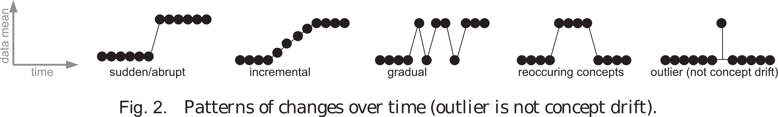
[1] Gama, J., Žliobaitė, I., Bifet, A., Pechenizkiy, M., & Bouchachia, A. (2014). "A survey on concept drift adaptation." ACM computing surveys (CSUR), 46(4), 1-37.
</small></small></small>
libraries
In [2]:
Copied!
import numpy as np
import pandas as pd

#https://scikit-multiflow.github.io/scikit-multiflow/documentation.html#learning-methods
from skmultiflow.drift_detection import DDM
from skmultiflow.drift_detection.eddm import EDDM
from skmultiflow.drift_detection import PageHinkley
from skmultiflow.drift_detection.adwin import ADWIN
from skmultiflow.evaluation import EvaluateHoldout

from skmultiflow.meta import AdaptiveRandomForest
from skmultiflow.trees import HoeffdingTree
from skmultiflow.trees import HAT
from skmultiflow.evaluation import EvaluatePrequential

from skmultiflow.data import DataStream

from sklearn.preprocessing import StandardScaler
from sklearn.metrics import classification_report
import matplotlib.pyplot as plt
%matplotlib inline
import glob
import numpy as np
import pandas as pd
#https://scikit-multiflow.github.io/scikit-multiflow/documentation.html#learning-methods
from skmultiflow.drift_detection import DDM
from skmultiflow.drift_detection.eddm import EDDM
from skmultiflow.drift_detection import PageHinkley
from skmultiflow.drift_detection.adwin import ADWIN
from skmultiflow.evaluation import EvaluateHoldout
from skmultiflow.meta import AdaptiveRandomForest
from skmultiflow.trees import HoeffdingTree
from skmultiflow.trees import HAT
from skmultiflow.evaluation import EvaluatePrequential
from skmultiflow.data import DataStream
from sklearn.preprocessing import StandardScaler
from sklearn.metrics import classification_report
import matplotlib.pyplot as plt
%matplotlib inline
import glob
Create a Workshop TEP dataset wih imbalanced classes for stream-based learning
In [10]:
Copied!
dataset = pd.read_csv('workshop_dataset.csv',index_col=False)
dataset_testing = pd.read_csv('workshop_dataset_stream_testing.csv',index_col=False)
dataset_orig = pd.concat([dataset,dataset_testing]).reset_index(drop=True)
test_size_orig = len(dataset_testing)
training_size_orig = len(dataset)

dataset_shuffled = pd.read_csv('workshop_dataset.csv',index_col=False).sample(frac=1).reset_index(drop=True)
col_names = dataset.columns.tolist()
test_size = len(dataset)//10
training_size = len(dataset) - test_size
dataset = pd.read_csv('workshop_dataset.csv',index_col=False)
dataset_testing = pd.read_csv('workshop_dataset_stream_testing.csv',index_col=False)
dataset_orig = pd.concat([dataset,dataset_testing]).reset_index(drop=True)
test_size_orig = len(dataset_testing)
training_size_orig = len(dataset)
dataset_shuffled = pd.read_csv('workshop_dataset.csv',index_col=False).sample(frac=1).reset_index(drop=True)
col_names = dataset.columns.tolist()
test_size = len(dataset)//10
training_size = len(dataset) - test_size
1. Concept Drift Detection
In [56]:
Copied!
# magnitude of row vectors - concept drift detectors take as input single value not list/vector
#cd_data = dataset[dataset.columns[:-1]].apply(np.linalg.norm, axis=1).values
feature = 'xmeas_11'
cd_data = dataset[feature].values
# magnitude of row vectors - concept drift detectors take as input single value not list/vector
#cd_data = dataset[dataset.columns[:-1]].apply(np.linalg.norm, axis=1).values
feature = 'xmeas_11'
cd_data = dataset[feature].values
In [57]:
Copied!
adwin = ADWIN()
ddm = DDM()
eddm = EDDM()
ph = PageHinkley()

adwin_detected_changes = []
ddm_detected_changes = []
eddm_detected_changes = []
ph_detected_changes = []

for i in range(len(cd_data)):
    adwin.add_element(cd_data[i])
    ddm.add_element(cd_data[i])
    eddm.add_element(cd_data[i])
    ph.add_element(cd_data[i])
    if adwin.detected_change():
        adwin_detected_changes.append([i,cd_data[i]])
    if ddm.detected_change():
        ddm_detected_changes.append([i,cd_data[i]])
    if eddm.detected_change():
        eddm_detected_changes.append([i,cd_data[i]])
    if ph.detected_change():
        ph_detected_changes.append([i,cd_data[i]])

adwin_detected_changes = np.array(adwin_detected_changes)
ddm_detected_changes = np.array(ddm_detected_changes)
eddm_detected_changes = np.array(eddm_detected_changes)
ph_detected_changes = np.array(ph_detected_changes)
adwin = ADWIN()
ddm = DDM()
eddm = EDDM()
ph = PageHinkley()
adwin_detected_changes = []
ddm_detected_changes = []
eddm_detected_changes = []
ph_detected_changes = []
for i in range(len(cd_data)):
adwin.add_element(cd_data[i])
ddm.add_element(cd_data[i])
eddm.add_element(cd_data[i])
ph.add_element(cd_data[i])
if adwin.detected_change():
adwin_detected_changes.append([i,cd_data[i]])
if ddm.detected_change():
ddm_detected_changes.append([i,cd_data[i]])
if eddm.detected_change():
eddm_detected_changes.append([i,cd_data[i]])
if ph.detected_change():
ph_detected_changes.append([i,cd_data[i]])
adwin_detected_changes = np.array(adwin_detected_changes)
ddm_detected_changes = np.array(ddm_detected_changes)
eddm_detected_changes = np.array(eddm_detected_changes)
ph_detected_changes = np.array(ph_detected_changes)
In [60]:
Copied!
eddm_detected_changes
eddm_detected_changes
Out[60]:
array([], dtype=float64)
In [65]:
Copied!
fig, ax = plt.subplots(1, 1, figsize=(18, 3), facecolor='w', edgecolor='k')
fig.suptitle('Detected concept drifts in feature: '+ feature, size=20, y=1.12)
adwin_plot = ax.scatter(adwin_detected_changes[:,0], adwin_detected_changes[:,1], color='red', marker='X', label='adwin')
#ddm_plot = ax.scatter(ddm_detected_changes[:,0], ddm_detected_changes[:,1], color='yellow', marker='s', label='ddm')
#eddm_plot = ax.scatter(eddm_detected_changes[:,0], eddm_detected_changes[:,1], color='green', marker='D', label='eddm')
ph_plot = ax.scatter(ph_detected_changes[:,0], ph_detected_changes[:,1], color='purple', marker='o', label='ph')
feature_plot = ax.plot(cd_data, color = 'black', alpha=0.3)
ax.set_xlim([0,len(cd_data)])
ax.legend()
Out[65]:
<matplotlib.legend.Legend at 0x7f98f715bba8>

2. Classification pipeline
2.1 Holdout - follows batch machine learning logic, i.e. train incremetanlly models and test it on test dataset
2.2 Prequential - test-then-train
2.3 Real-world scenarios - model is incrementally trained and then incremetally tested by comparing predicted labels to ground truth
2.1. Holdout evaluation - without shuffling
In [11]:
Copied!
HAT.reset()
#HAT = HAT()

samples = dataset_orig.drop(columns=['fault_id'])
labels  = dataset_orig['fault_id'].to_frame()

stream = DataStream(data = samples, y = labels)
stream.prepare_for_use()

evaluator = EvaluateHoldout(max_samples=100000,
                            max_time=7200,
                            n_wait=100,
                            batch_size=100,
                            test_size=training_size_orig,
                            output_file='HAT_holdout_noshuffling.csv',
                            metrics=['precision','recall','f1'])
evaluator.evaluate(stream=stream, model=[HAT], model_names=['HAT'])
HAT.reset()
#HAT = HAT()
samples = dataset_orig.drop(columns=['fault_id'])
labels = dataset_orig['fault_id'].to_frame()
stream = DataStream(data = samples, y = labels)
stream.prepare_for_use()
evaluator = EvaluateHoldout(max_samples=100000,
max_time=7200,
n_wait=100,
batch_size=100,
test_size=training_size_orig,
output_file='HAT_holdout_noshuffling.csv',
metrics=['precision','recall','f1'])
evaluator.evaluate(stream=stream, model=[HAT], model_names=['HAT'])
Holdout Evaluation
Evaluating 1 target(s).
Separating 20232 holdout samples.
Evaluating...
 #################### [100%] [5749.74s]
Processed samples: 31732
Mean performance:
HAT - Precision: 1.0000
HAT - Recall: 0.4075
HAT - F1 score: 0.5790
Out[11]:
[HAT(binary_split=False, grace_period=200, leaf_prediction='nba',
     max_byte_size=33554432, memory_estimate_period=1000000, nb_threshold=0,
     no_preprune=False, nominal_attributes=None, remove_poor_atts=False,
     split_confidence=1e-07, split_criterion='info_gain',
     stop_mem_management=False, tie_threshold=0.05)]
2.2. Holdout evaluation - with shuffling
In [4]:
Copied!
HAT.reset()
samples = dataset_shuffled.drop(columns=['fault_id'])
labels  = dataset_shuffled['fault_id'].to_frame()

stream = DataStream(data = samples, y = labels)
stream.prepare_for_use()

evaluator = EvaluateHoldout(max_samples=100000,
                            max_time=7200,
                            n_wait=100,
                            batch_size=100,
                            test_size=training_size,
                            output_file='HAT_holdout.csv',
                            metrics=['precision','recall','f1'])
evaluator.evaluate(stream=stream, model=[HAT], model_names=['HAT'])
HAT.reset()
samples = dataset_shuffled.drop(columns=['fault_id'])
labels = dataset_shuffled['fault_id'].to_frame()
stream = DataStream(data = samples, y = labels)
stream.prepare_for_use()
evaluator = EvaluateHoldout(max_samples=100000,
max_time=7200,
n_wait=100,
batch_size=100,
test_size=training_size,
output_file='HAT_holdout.csv',
metrics=['precision','recall','f1'])
evaluator.evaluate(stream=stream, model=[HAT], model_names=['HAT'])
Holdout Evaluation
Evaluating 1 target(s).
Separating 18209 holdout samples.
Evaluating...
 #################### [100%] [2358.34s]
Processed samples: 20309
Mean performance:
HAT - Precision: 0.9990
HAT - Recall: 0.9983
HAT - F1 score: 0.9987
Out[4]:
[HAT(binary_split=False, grace_period=200, leaf_prediction='nba',
     max_byte_size=33554432, memory_estimate_period=1000000, nb_threshold=0,
     no_preprune=False, nominal_attributes=None, remove_poor_atts=False,
     split_confidence=1e-07, split_criterion='info_gain',
     stop_mem_management=False, tie_threshold=0.05)]
2.3. Prequential evaluation
In [5]:
Copied!
HAT.reset()
evaluator = EvaluatePrequential(n_wait=100,
                                batch_size=100,
                                pretrain_size=100,
                                output_file='HAT_prequential.csv',
                                metrics=['precision','recall','f1'])
evaluator.evaluate(stream=stream, model=HAT, model_names=['HAT'])
HAT.reset()
evaluator = EvaluatePrequential(n_wait=100,
batch_size=100,
pretrain_size=100,
output_file='HAT_prequential.csv',
metrics=['precision','recall','f1'])
evaluator.evaluate(stream=stream, model=HAT, model_names=['HAT'])
Prequential Evaluation
Evaluating 1 target(s).
Pre-training on 100 sample(s).
Evaluating...
 #################### [100%] [361.08s]
Processed samples: 20300
Mean performance:
HAT - Precision: 0.9634
HAT - Recall: 0.9351
HAT - F1 score: 0.9490
Out[5]:
[HAT(binary_split=False, grace_period=200, leaf_prediction='nba',
     max_byte_size=33554432, memory_estimate_period=1000000, nb_threshold=0,
     no_preprune=False, nominal_attributes=None, remove_poor_atts=False,
     split_confidence=1e-07, split_criterion='info_gain',
     stop_mem_management=False, tie_threshold=0.05)]
In [75]:
Copied!
# skmultiflow saves results to file with leading 5 lines containing configuraiton of evaluation, learner etc
# skmultiflow also did not evaluate last 200 samples
# for the sake of comparisson we shrink the MOA results
# accuracy in MOA is in % and in skmultiflow fraction
HAT_holdout_results = pd.read_csv('HAT_holdout.csv',skiprows=[0,1,2,3,4],index_col='id')
HAT_prequential_results = pd.read_csv('HAT_prequential.csv',skiprows=[0,1,2,3,4],index_col='id')
In [88]:
Copied!
fig, ax = plt.subplots(1, 1, figsize=(18, 3), facecolor='w', edgecolor='k')
fig.suptitle('Holdout vs Prequential evaluation results, mean(f1)', size=20, y=1.12)
HAT_holdout_results['mean_f1_[HAT]'].plot(ax=ax, label='holdout', linewidth=3)
HAT_prequential_results['mean_f1_[HAT]'].plot(ax=ax, label='prequential', linewidth=3)
ax.vlines(training_size,0,1.5, label='end of training')
ax.set_ylim([0,1.1])
ax.set_xlabel('sample id')
ax.set_ylabel('score')
ax.legend()
Out[88]:
<matplotlib.legend.Legend at 0x7f98f6e49fd0>

2.4. Real-world scenario
2.4.1. Incremental approach
2.4.1.1. Train
In [67]:
Copied!
HAT.reset()

samples_train = dataset_shuffled.drop(columns=['fault_id']).values[:training_size]
labels_train  = dataset_shuffled['fault_id'].to_frame().values.flatten()[:training_size]

stream_train = DataStream(data=samples_train, y=labels_train)
stream_train.prepare_for_use()

for sample in range(len(labels_train)):
    X, Y = stream_train.next_sample()
    HAT.partial_fit(X, Y)
HAT.reset()
samples_train = dataset_shuffled.drop(columns=['fault_id']).values[:training_size]
labels_train = dataset_shuffled['fault_id'].to_frame().values.flatten()[:training_size]
stream_train = DataStream(data=samples_train, y=labels_train)
stream_train.prepare_for_use()
for sample in range(len(labels_train)):
X, Y = stream_train.next_sample()
HAT.partial_fit(X, Y)
2.4.1.2. Test
In [68]:
Copied!
samples_test = dataset_shuffled.drop(columns=['fault_id']).values[training_size:]
labels_test  = dataset_shuffled['fault_id'].to_frame().values.flatten()[training_size:]

stream_test = DataStream(data = samples_test, y = labels_test)
stream_test.prepare_for_use()

labels_test_predicted = []
for sample in range(len(labels_test)):
    X, Y = stream_test.next_sample()
    Y_pred = HAT.predict(X)
    labels_test_predicted.extend(HAT.predict(X))

print('Classification report :\n' + str(classification_report(labels_test, labels_test_predicted)))
samples_test = dataset_shuffled.drop(columns=['fault_id']).values[training_size:]
labels_test = dataset_shuffled['fault_id'].to_frame().values.flatten()[training_size:]
stream_test = DataStream(data = samples_test, y = labels_test)
stream_test.prepare_for_use()
labels_test_predicted = []
for sample in range(len(labels_test)):
X, Y = stream_test.next_sample()
Y_pred = HAT.predict(X)
labels_test_predicted.extend(HAT.predict(X))
print('Classification report :\n' + str(classification_report(labels_test, labels_test_predicted)))
Classification report :
              precision    recall  f1-score   support

           0       0.07      0.25      0.11        12
           1       0.91      0.72      0.80       141
           2       0.99      0.88      0.93       121
           3       0.25      0.51      0.34       109
           4       0.88      0.88      0.88       128
           5       0.27      0.14      0.18       132
           6       1.00      0.88      0.93       120
           7       1.00      0.86      0.92        71
           8       0.63      0.59      0.61       140
           9       0.22      0.37      0.28        95
          10       0.56      0.39      0.46       162
          11       0.67      0.67      0.67        24
          12       0.68      0.62      0.65       115
          13       0.60      0.60      0.60        78
          14       0.82      0.80      0.81       120
          15       0.21      0.18      0.19        84
          16       0.14      0.20      0.16        41
          17       0.83      0.64      0.72        67
          18       0.38      0.44      0.41        18
          19       0.36      0.61      0.45        72
          20       0.71      0.59      0.65       113
          21       1.00      0.58      0.74        60

    accuracy                           0.59      2023
   macro avg       0.60      0.56      0.57      2023
weighted avg       0.65      0.59      0.61      2023
2.4.2. Bulk approach
In [70]:
Copied!
HAT.reset()
HAT.fit(samples_train,labels_train.flatten())
labels_test_predicted = HAT.predict(samples_test)
print('Classification report :\n' + str(classification_report(labels_test, labels_test_predicted)))
HAT.reset()
HAT.fit(samples_train,labels_train.flatten())
labels_test_predicted = HAT.predict(samples_test)
print('Classification report :\n' + str(classification_report(labels_test, labels_test_predicted)))
Classification report :
              precision    recall  f1-score   support

           0       0.07      0.25      0.11        12
           1       0.91      0.72      0.80       141
           2       0.99      0.88      0.93       121
           3       0.25      0.51      0.34       109
           4       0.88      0.88      0.88       128
           5       0.27      0.14      0.18       132
           6       1.00      0.88      0.93       120
           7       1.00      0.86      0.92        71
           8       0.63      0.59      0.61       140
           9       0.22      0.37      0.28        95
          10       0.56      0.39      0.46       162
          11       0.67      0.67      0.67        24
          12       0.68      0.62      0.65       115
          13       0.60      0.60      0.60        78
          14       0.82      0.80      0.81       120
          15       0.21      0.18      0.19        84
          16       0.14      0.20      0.16        41
          17       0.83      0.64      0.72        67
          18       0.38      0.44      0.41        18
          19       0.36      0.61      0.45        72
          20       0.71      0.59      0.65       113
          21       1.00      0.58      0.74        60

    accuracy                           0.59      2023
   macro avg       0.60      0.56      0.57      2023
weighted avg       0.65      0.59      0.61      2023